1
2
3

# Initialize Otter
import otter
grader = otter.Notebook("lab03.ipynb")

Lab 3: Data Cleaning and EDA

In this lab you will be working on visualizing a dataset from the City of Berkeley containing data on calls to the Berkeley Police Department. Information about the dataset can be found at this link.

Content Warning

This lab includes an analysis of crime in Berkeley. If you feel uncomfortable with this topic, please contact your GSI or the instructors.

Setup

In this lab, we’ll perform Exploratory Data Analysis and learn some preliminary tips for working with matplotlib (a Python plotting library). Note that we configure a custom default figure size. Virtually every default aspect of matplotlib can be customized.

Collaborators: list names here

1
2
3
4
5
6
7

import pandas as pd
import numpy as np
import zipfile
import matplotlib
import matplotlib.pyplot as plt

plt.rcParams['figure.figsize'] = (12, 9)

1
2

fig = plt.figure()
plt.show(fig)

<Figure size 1200x900 with 0 Axes>

Part 1: Acquire the Data

1. Obtain data
To retrieve the dataset, we will use the ds100_utils.fetch_and_cache utility.

1
2
3
4
5
6
7
8
9

# just run this cell
import ds100_utils

data_dir = 'data'
data_url = 'http://www.ds100.org/sp22/resources/assets/datasets/lab03_data_sp22.zip'
file_name = 'lab03_data_sp22.zip'

dest_path = ds100_utils.fetch_and_cache(data_url=data_url, file=file_name, data_dir=data_dir)
print(f'Located at {dest_path}')

Using cached version that was downloaded (UTC): Sun Jul 28 01:04:24 2024
Located at data\lab03_data_sp22.zip

2. Unzip file
We will now directly unzip the ZIP archive and start working with the uncompressed files.

1
2
3

# just run this cell
my_zip = zipfile.ZipFile(dest_path, 'r')
my_zip.extractall(data_dir)

Note: There is no single right answer regarding whether to work with compressed files in their compressed state or to uncompress them on disk permanently. For example, if you need to work with multiple tools on the same files, or write many notebooks to analyze them—and they are not too large—it may be more convenient to uncompress them once. But you may also have situations where you find it preferable to work with the compressed data directly.

Python gives you tools for both approaches, and you should know how to perform both tasks in order to choose the one that best suits the problem at hand.

3. View files

Now, we’ll use the os package to list all files in the data directory. os.walk() recursively traverses the directory, and os.path.join() creates the full pathname of each file.

If you’re interested in learning more, check out the Python3 documentation pages for os.walk (link) and os.path (link).

We use Python 3 format strings to nicely format the printed variables dpath and fpath.

 1
 2
 3
 4
 5
 6
 7
 8
 9
10
11
12
13
14

# just run this cell
# two for loop in the same time... ? not that funny yet?
import os

for root, directories, filenames in os.walk(data_dir):
    # first, print out all directories ---> "secret"
    for directory in directories:
        dpath = os.path.join(root, directory)
        print(f"d {dpath}")
        
    # next, print out all files
    for filename in filenames:  
        fpath = os.path.join(root,filename)
        print(f"  {fpath}")

d data\secret
  data\ben_kurtovic.py
  data\Berkeley_PD_-_Calls_for_Service.csv
  data\dummy.txt
  data\hello_world.py
  data\lab03_data_sp22.zip
  data\secret\do_not_readme.md

In this Lab, we’ll be working with the Berkeley_PD_-_Calls_for_Service.csv file. Feel free to check out the other files, though.

Part 2: Clean and Explore the Data

Let’s now load the CSV file we have into a pandas.DataFrame object and start exploring the data.

1
2
3

# just run this cell
calls = pd.read_csv("data/Berkeley_PD_-_Calls_for_Service.csv")
calls.head()

We see that the fields include a case number, the offense type, the date and time of the offense, the “CVLEGEND” which appears to be related to the offense type, a “CVDOW” which has no apparent meaning, a date added to the database, and the location spread across four fields. We can read more about each field from the City of the Berkeley’s open dataset webpage.

Let’s also check some basic information about this DataFrame using the DataFrame.info (documentation) and DataFrame.describe methods (documentation).

1
2
3
4
5

# df.info() displays 
# name and type of each column,
# number of non-null entries, and
# size of dataframe
calls.info()

<class 'pandas.core.frame.DataFrame'>
RangeIndex: 2632 entries, 0 to 2631
Data columns (total 11 columns):
 #   Column          Non-Null Count  Dtype 
---  ------          --------------  ----- 
 0   CASENO          2632 non-null   int64 
 1   OFFENSE         2632 non-null   object
 2   EVENTDT         2632 non-null   object
 3   EVENTTM         2632 non-null   object
 4   CVLEGEND        2632 non-null   object
 5   CVDOW           2632 non-null   int64 
 6   InDbDate        2632 non-null   object
 7   Block_Location  2632 non-null   object
 8   BLKADDR         2612 non-null   object
 9   City            2632 non-null   object
 10  State           2632 non-null   object
dtypes: int64(2), object(9)
memory usage: 226.3+ KB

Note that the BLKADDR column only has 2612 non-null entries, while the other columns all have 2632 entries. This is because the .info() method only counts non-null entries.

1

calls.describe()

Notice that the functions above reveal type information for the columns, as well as some basic statistics about the numerical columns found in the DataFrame. However, we still need more information about what each column represents. Let’s explore the data further in Question 1.

Before we go over the fields to see their meanings, the cell below will verify that all the events happened in Berkeley by grouping on the City and State columns. You should see that all of our data falls into one group.

1

calls.groupby(["City","State"]).count()

When we called head() on the Dataframe calls, it seemed like OFFENSE and CVLEGEND both contained information about the type of event reported. What is the difference in meaning between the two columns? One way to probe this is to look at the value_counts for each Series.

1

calls['OFFENSE'].value_counts().head(10)

OFFENSE
THEFT MISD. (UNDER $950)    559
VEHICLE STOLEN              277
BURGLARY AUTO               218
THEFT FELONY (OVER $950)    215
DISTURBANCE                 204
BURGLARY RESIDENTIAL        178
VANDALISM                   166
THEFT FROM AUTO             163
ASSAULT/BATTERY MISD.       116
ROBBERY                      90
Name: count, dtype: int64

1

calls['CVLEGEND'].value_counts().head(10)

CVLEGEND
LARCENY                   782
MOTOR VEHICLE THEFT       277
BURGLARY - VEHICLE        218
DISORDERLY CONDUCT        204
BURGLARY - RESIDENTIAL    178
VANDALISM                 166
LARCENY - FROM VEHICLE    163
ASSAULT                   150
FRAUD                      93
ROBBERY                    90
Name: count, dtype: int64

It seems like OFFENSE is more specific than CVLEGEND, e.g. “LARCENY” vs. “THEFT FELONY (OVER $950)”. If you’re unfamiliar with the term, “larceny” is a legal term for theft of personal property.

To get a sense of how many subcategories there are for each OFFENSE, we will set calls_by_cvlegend_and_offense equal to a multi-indexed series where the data is first indexed on the CVLEGEND and then on the OFFENSE, and the data is equal to the number of offenses in the database that match the respective CVLEGEND and OFFENSE. As you can see, calls_by_cvlegend_and_offense["LARCENY", "THEFT FROM PERSON"] returns 8 which means there are 8 instances of larceny with offense of type “THEFT FROM PERSON” in the database.

1
2

calls_by_cvlegend_and_offense = calls.groupby(["CVLEGEND", "OFFENSE"]).size()
calls_by_cvlegend_and_offense["LARCENY", "THEFT FROM PERSON"]

np.int64(8)

Question 1

In the cell below, set answer1 equal to a list of strings corresponding to the possible values (which means unique 🤔 ) for OFFENSE when CVLEGEND is “LARCENY”. You can type the answer manually, or you can create an expression that automatically extracts the names.

1
2

answer1 = list(calls[calls['CVLEGEND'] == 'LARCENY']['OFFENSE'].unique())
answer1

['THEFT MISD. (UNDER $950)', 'THEFT FELONY (OVER $950)', 'THEFT FROM PERSON']

1

grader.check("q1")

q1

Part 3: Visualize the Data

Matplotlib demo

You’ve seen some matplotlib in this class already, but now we will explain how to work with the object-oriented plotting API mentioned in this matplotlib.pyplot tutorial useful. In matplotlib, plotting occurs on a set of Axes which are associated with a Figure. An analogy is that on a blank canvas (Figure), you choose a location to plot (Axes) and then fill it in (plot).

There are two approaches to labeling and manipulating figure contents, which we’ll discuss below. Approach 1 is closest to the plotting paradigm of MATLAB, the namesake of matplotlib; Approach 2 is also common because many matplotlib-based packages (such as Seaborn) explicitly return the current set of axes after plotting data. Both are essentially equivalent, and at the end of this class you’ll be comfortable with both.

Approach 1: matplotlib (or Seaborn) will auto-plot onto the current set of Axes or (if none exists) create a new figure/set of default axes. You can plot data using methods from plt, which is shorthand for the matplotlib.pyplot package. Then subsequent plt calls all edit the same set of default-created axes.

Approach 2:
After creating the initial plot, you can also use plt.gca() to explicitly get the current set of axes, and then edit those specific axes using axes methods. Note the method naming is slightly different!

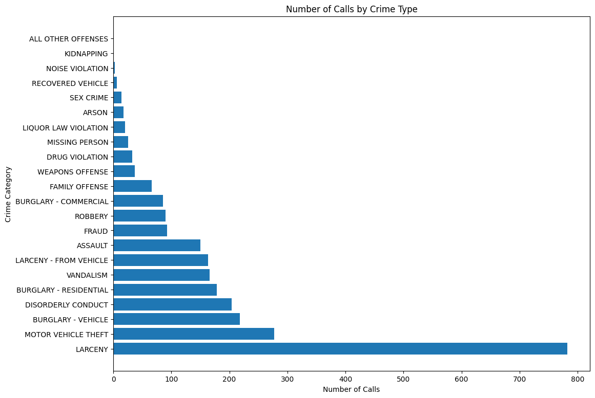
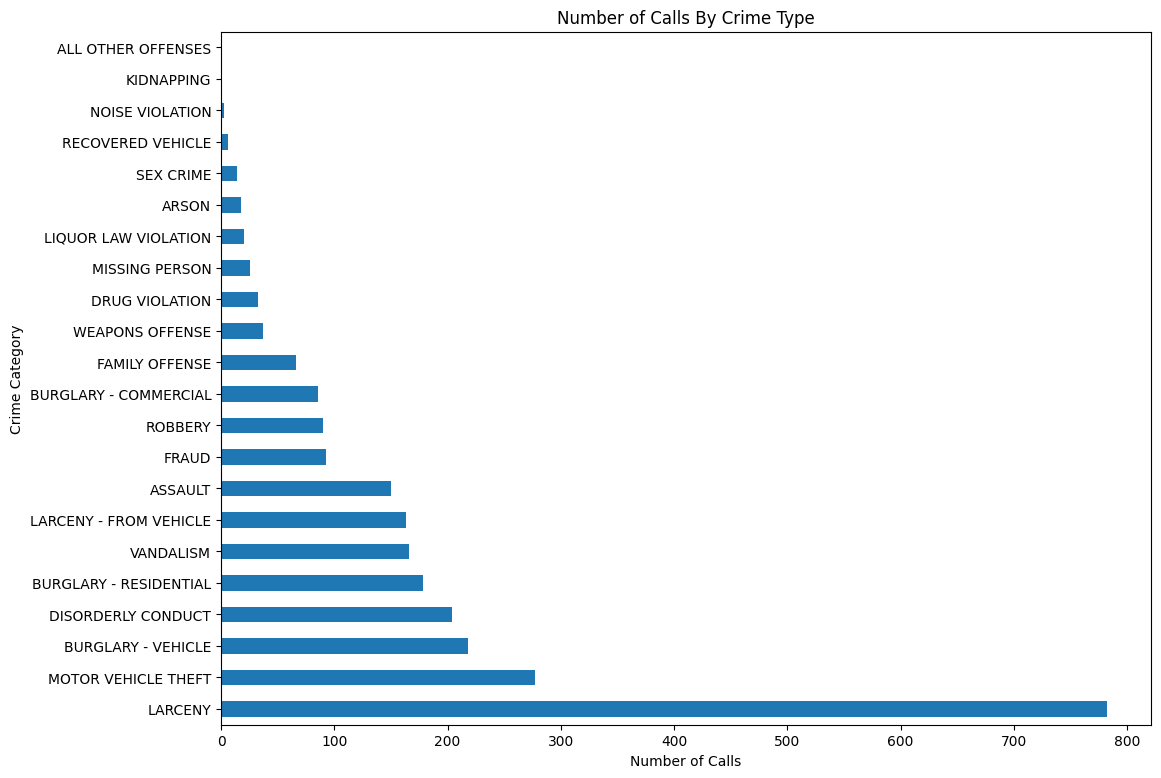
As an example of the built-in plotting functionality of pandas, the following example uses plot method of the Series class to generate a barh plot type to visually display the value counts for CVLEGEND.

There are also many other plots that we will explore throughout the lab.

Side note: Pandas also offers basic functionality for plotting. For example, the DataFrame and Series classes both have a plot method, which uses matplotlib under the hood. For now we’ll focus on matplotlib itself so you get used to the syntax, but just know that convenient Pandas plotting methods exist for your own future data science exploration.

Below, we show both approaches by generating a horizontal bar plot to visually display the value counts for CVLEGEND. See the barhdocumentation for more details.

 1
 2
 3
 4
 5
 6
 7
 8
 9
10
11
12
13
14
15
16
17
18
19
20
21
22

# DEMO CELL: assign demo to 1 or 2.
demo = 1

calls_cvlegend = calls['CVLEGEND'].value_counts()

if demo == 1:
    plt.barh(calls_cvlegend.index, calls_cvlegend) # creates figure and axes (y,x) not (x,y)!
    print(f"Demo {demo}: Using plt methods to update plot")
    plt.ylabel("Crime Category")               # uses most recently plotted axes
    plt.xlabel("Number of Calls")
    plt.title("Number of Calls by Crime Type")
elif demo == 2:
    print(f"Demo {demo}: Using axes methods to update plot")
    plt.barh(calls_cvlegend.index, calls_cvlegend) # creates figure and axes
    ax = plt.gca()
    ax.set_ylabel("Crime Category")
    ax.set_xlabel("Number of Calls")
    ax.set_title("Axes methods: Number of Calls by Crime Type")
else:
    print("Error: Please assign the demo variable to 1 or 2.")

plt.show()

Demo 1: Using plt methods to update plot

An Additional Note on Plotting in Jupyter Notebooks

You may have noticed that many of our plotting code cells end with a semicolon ; or plt.show(). The former prevents any extra output from the last line of the cell; the latter explicitly returns (and outputs) the figure. Try adding this to your own code in the following questions!

Question 2

Now it is your turn to make a plot using matplotlib. Let’s start by transforming the data so that it is easier to work with.

The CVDOW field isn’t named helpfully and it is hard to see the meaning from the data alone. According to the website linked at the top of this notebook, CVDOW is actually indicating the day that events happened. 0->Sunday, 1->Monday … 6->Saturday.

Question 2a

Add a new column Day into the calls dataframe that has the string weekday (eg. ‘Sunday’) for the corresponding value in CVDOW. For example, if the first 3 values of CVDOW are [3, 6, 0], then the first 3 values of the Day column should be ["Wednesday", "Saturday", "Sunday"].

Hint: Try using the Series.map function on calls["CVDOW"]. Can you assign this to the new column calls["Day"]?

1
2
3
4
5

days = ["Sunday", "Monday", "Tuesday", "Wednesday", "Thursday", "Friday", "Saturday"]
day_indices = range(7)
indices_to_days_dict = dict(zip(day_indices, days)) # Should look like {0:"Sunday", 1:"Monday", ..., 6:"Saturday"}

calls["Day"] = calls["CVDOW"].map(indices_to_days_dict)

1

grader.check("q2a")

q2a

1
2
3
4
5

# just run this example cell
ax = calls['CVLEGEND'].value_counts().plot(kind='barh')
ax.set_ylabel("Crime Category")
ax.set_xlabel("Number of Calls")
ax.set_title("Number of Calls By Crime Type");

Challenge (OPTIONAL): You could also accomplish this part as a table left join with pd.merge (documentation), instead of using Series.map. You would need to merge calls with a new dataframe that just contains the days of the week. If you have time, try it out in the below cell!

merge操作在接下来的lab有详细介绍！😉

1
2
3
4

# scratch space for optional challenge
dow_df = pd.DataFrame(days, columns=["Day"])

...

Ellipsis

Question 2b

Now let’s look at the EVENTTM column which indicates the time for events. Since it contains hour and minute information, let’s extract the hour info and create a new column named Hour in the calls dataframe. You should save the hour as an int.

Hint: Your code should only require one line.
Hint 2: The vectorized Series.str[ind] performs integer indexing on an array entry.

1
2

calls["Hour"] = calls["EVENTTM"].str.split(" ").str[0].str.split(":").str[0].astype(int)
calls["Hour"]

0       10
1       10
2       12
3       17
4        6
        ..
2627    12
2628    15
2629     0
2630    18
2631     2
Name: Hour, Length: 2632, dtype: int64

1

grader.check("q2b")

Question 2c

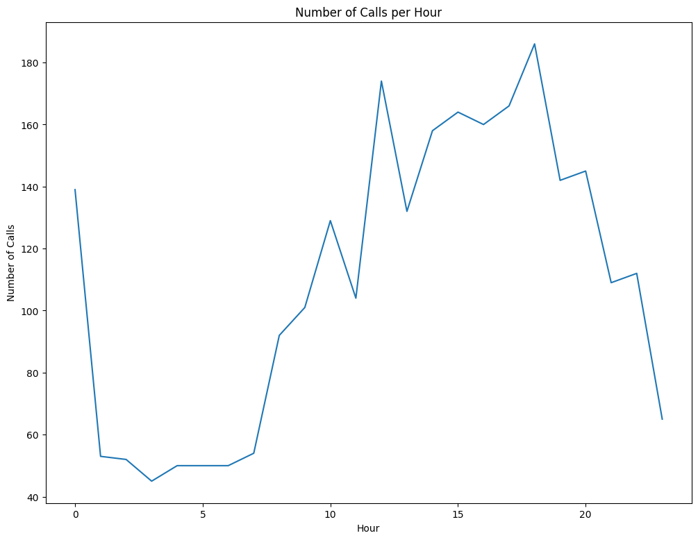
Using matplotlib, construct a line plot with the count of the number of calls (entries in the table) for each hour of the day ordered by the time (eg. 12:00 AM, 1:00 AM, …). Please use the provided variable hours in your answer. Be sure that your axes are labeled and that your plot is titled.

Hint: Check out the plt.plot method in the matplotlib tutorial, as well as our demo above.

 1
 2
 3
 4
 5
 6
 7
 8
 9
10

hours = list(range(24))
calls_index = calls['Hour'].value_counts().sort_index()
# calls_index
plt.plot(hours, calls_index)
plt.xlabel("Hour")
plt.ylabel("Number of Calls")
plt.title("Number of Calls per Hour")

# Leave this for grading purposes
ax_3d = plt.gca()

1

grader.check("q2c")

q2c

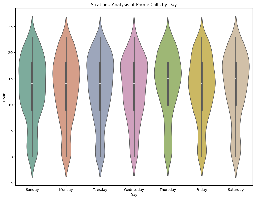
To better understand the time of day a report occurs we could stratify the analysis by the day of the week. To do this we will use violin plots (a variation of a box plot), which you will learn in more detail next week.

For now, just know that a violin plot shows an estimated distribution of quantitative data (e.g., distribution of calls by hour) over a categorical variable (day of the week). More calls occur in hours corresponding to the fatter part of each violin; the median hour of all calls in a particular day is marked by the white dot in the corresponding violin.

1
2
3
4
5
6
7
8

# for now, just run this cell.
# we will learn the seaborn visualization library next week.

import seaborn as sns
ax = sns.violinplot(data=calls.sort_values("CVDOW"),
                    x="Day", y="Hour",
                    saturation=0.5, palette="Set2")
ax.set_title("Stratified Analysis of Phone Calls by Day");

C:\Users\86135\AppData\Local\Temp\ipykernel_19968\4044437892.py:5: FutureWarning: 

Passing `palette` without assigning `hue` is deprecated and will be removed in v0.14.0. Assign the `x` variable to `hue` and set `legend=False` for the same effect.

  ax = sns.violinplot(data=calls.sort_values("CVDOW"),

Question 2d

Based on your line plot and our violin plot above, what observations can you make about the patterns of calls? Here are some dimensions to consider:

• Are there more calls in the day or at night?
• What are the most and least popular times?
• Do call patterns vary by day of the week?

Question 3

In this last part of the lab, let’s extract the GPS coordinates (latitude, longitude) from the Block_Location of each record.

1
2

# an example block location entry
calls.loc[4, 'Block_Location']

'2700 BLOCK GARBER ST\nBerkeley, CA\n(37.86066, -122.253407)'

Question 3a: Regular Expressions

Use regular expressions to create a dataframe calls_lat_lon that has two columns titled Lat and Lon, containing the respective latitude and longitude of each record in calls. You should use the Block_Location column to extract the latitude and longitude coordinates.

Hint: Check out the Series.str.extract documentation.

1
2
3
4
5
6
7

calls_lat_lon = calls['Block_Location'].str.extract(r'(\d+\.\d+),\s([-]*\d+\.\d+)')
# 注意捕获组涵盖范围！
calls_lat_lon.columns = ['Lat', 'Lon']

calls_lat_lon.head(10)

len(calls_lat_lon)

2632

1

grader.check("q3a")

q3a

Question 3b: Join Tables

Let’s include the GPS data into our calls data. In the below cell, use calls_lat_lon to add two new columns called Lat and Lon to the calls dataframe.

Hint: pd.merge (documentation) could be useful here. Note that the order of records in calls and calls_lat_lon are the same.

 1
 2
 3
 4
 5
 6
 7
 8
 9
10
11

import pandas as pd

# 创建两个长度相同的DataFrame
df1 = pd.DataFrame({'A': [1, 2, 3], 'B': [4, 5, 6]})
df2 = pd.DataFrame({'C': [7, 8, 9], 'D': [10, 11, 12]})

# 基于索引合并

# 使用'Key'列合!
merged_df = pd.merge(df1, df2, left_index=True, right_index=True)  # 根据你的需要选择合并类型
print(merged_df)

   A  B  C   D
0  1  4  7  10
1  2  5  8  11
2  3  6  9  12

1
2
3
4
5
6
7

# # 用merge合并两个dataframe，注意此时没有共同列！只能索引拼接！
# print(calls.shape)
# print(calls_lat_lon.shape)
calls = pd.merge(calls, calls_lat_lon, left_index=True, right_index=True)

# print(calls.shape)
calls.sample(5)      # random rows

1

grader.check("q3b")

q3b

Question 3c: Check for Missing Values

It seems like every record has valid GPS coordinates:

1
2
3

# just run this cell
# fraction of valid lat/lon entries
(~calls[["Lat", "Lon"]].isna()).mean()

Lat    1.0
Lon    1.0
dtype: float64

However, a closer examination of the data reveals something else. Here’s the first few records of our data again:

1

calls.head(5)

There is another field that tells us whether we have a valid Block_Location entry per record—i.e., with GPS coordinates (latitude, longitude) that match the listed block location. What is it?

In the below cell, use the field you found to create a new dataframe, missing_lat_lon, that contains only the rows of calls that have invalid latitude and longitude data. Your new dataframe should have all the same columns of calls.

1
2
3
4

missing_lat_lon = calls[calls['Lat'] == '37.869058'] # 理论上应该是lat和lon，但是这里只取了lat，然后注意类型隐式转换！
missing_lat_lon.head()

# print(missing_lat_lon.shape)

1

grader.check("q3c")

Question 3d: Check Missing Values

Now let us explore if there is a pattern to which types of records have missing latitude and longitude entries.

We’ve implemented the plotting code for you below, but read through it and verify you understand what we’re doing (we’ve thrown in a bonus plt.subplots() call, documentation here).

 1
 2
 3
 4
 5
 6
 7
 8
 9
10
11
12
13
14
15
16
17

# just run this cell
missing_by_time = (pd.to_datetime(missing_lat_lon['EVENTDT'])
                   .value_counts()
                   .sort_index()
                  )
missing_by_crime = (missing_lat_lon['CVLEGEND']
                    .value_counts() 
                    / calls['CVLEGEND'].value_counts()
                   ).dropna().sort_values(ascending=False)

fig, ax = plt.subplots(2)
ax[0].bar(missing_by_time.index, missing_by_time)
ax[0].set_ylabel("Calls with Missing Data")
ax[1].barh(missing_by_crime.index, missing_by_crime)
ax[1].set_xlabel("Fraction of Missing Data per Event Type")
fig.suptitle("Characteristics of Missing Lat/Lon Data")
plt.show()

C:\Users\86135\AppData\Local\Temp\ipykernel_19968\1218153592.py:2: UserWarning: Could not infer format, so each element will be parsed individually, falling back to `dateutil`. To ensure parsing is consistent and as-expected, please specify a format.
  missing_by_time = (pd.to_datetime(missing_lat_lon['EVENTDT'])

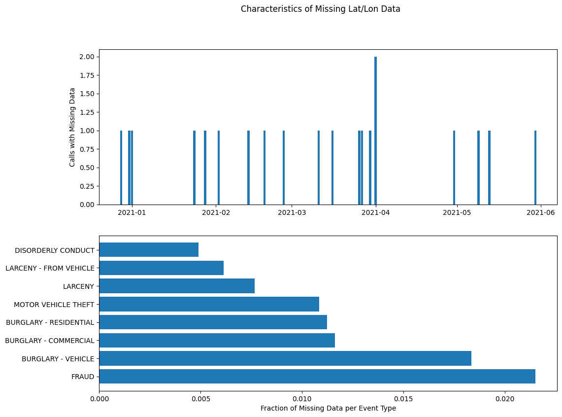
Based on the plots above, are there any patterns among entries that are missing latitude/longitude data? The dataset information linked at the top of this notebook may also give more context.

Type your answer here, replacing this text.

Question 3d: Explore

The below cell plots a map of phonecalls by GPS coordinates (latitude, longitude); we drop missing location data.

1
2
3
4
5
6
7
8
9

# just run this cell
import folium
import folium.plugins

SF_COORDINATES = (37.87, -122.28)
sf_map = folium.Map(location=SF_COORDINATES, zoom_start=13)
locs = calls.drop(missing_lat_lon.index)[['Lat', 'Lon']].astype('float').values
heatmap = folium.plugins.HeatMap(locs.tolist(), radius=10)
sf_map.add_child(heatmap)